PyEGRO.sensitivity.SApce Usage Examples¶

This document provides examples of how to use the PyEGRO.sensitivity.SApce module for sensitivity analysis using Polynomial Chaos Expansion (PCE).

Table of Contents¶

Quick Start
Basic Setup
Running the Analysis
Working with Different Models
Using a Direct Function
Using a Surrogate Model
Example Applications
Ishigami Function
Rosenbrock Function
Borehole Function
Circuit Design Problem

Quick Start¶

Basic Setup¶

The simplest way to use the PyEGRO.sensitivity.SApce module is with the convenience function run_sensitivity_analysis.

import numpy as np
from PyEGRO.sensitivity.SApce import run_sensitivity_analysis

# Define a simple test function
def test_function(X):
    """
    Simple quadratic function with interactions.
    """
    x1 = X[:, 0]
    x2 = X[:, 1]
    x3 = X[:, 2]

    return x1**2 + 0.5*x2**2 + 0.1*x3**2 + 0.7*x1*x2 + 0.2*x2*x3

# Define data_info with variable definitions
data_info = {
    'variables': [
        {
            'name': 'x1',
            'vars_type': 'design_vars',
            'distribution': 'uniform',
            'range_bounds': [-1, 1],
            'description': 'First input variable'
        },
        {
            'name': 'x2',
            'vars_type': 'design_vars',
            'distribution': 'uniform',
            'range_bounds': [-1, 1],
            'description': 'Second input variable'
        },
        {
            'name': 'x3',
            'vars_type': 'design_vars',
            'distribution': 'uniform',
            'range_bounds': [-1, 1],
            'description': 'Third input variable'
        }
    ]
}

# Save data_info to a JSON file
import json
import os

os.makedirs("DATA_PREPARATION", exist_ok=True)
with open("DATA_PREPARATION/data_info.json", 'w') as f:
    json.dump(data_info, f)

# Run the analysis
results_df = run_sensitivity_analysis(
    data_info_path="DATA_PREPARATION/data_info.json",
    true_func=test_function,
    polynomial_order=3,
    num_samples=500,
    output_dir="RESULT_SA_QUADRATIC",
    random_seed=42,
    show_progress=True
)

# Print the results
print("\nSensitivity Indices:")
print(results_df)

Running the Analysis¶

For more control over the analysis process, you can use the PCESensitivityAnalysis class directly:

from PyEGRO.sensitivity.SApce import PCESensitivityAnalysis

# Initialize the analysis
analyzer = PCESensitivityAnalysis(
    data_info_path="DATA_PREPARATION/data_info.json",
    true_func=test_function,
    output_dir="RESULT_SA_DETAILED",
    show_variables_info=True,
    random_seed=42
)

# Run the analysis
results_df = analyzer.run_analysis(
    polynomial_order=4,  # Higher order for more accuracy
    num_samples=1000,
    show_progress=True
)

# Examine the summary statistics
import json
with open("RESULT_SA_DETAILED/analysis_summary.json", 'r') as f:
    summary = json.load(f)

print("\nAnalysis Summary:")
for key, value in summary.items():
    print(f"{key}: {value}")

Working with Different Models¶

Using a Direct Function¶

For analytical functions or inexpensive simulations, you can directly use the function for evaluations:

import numpy as np
from PyEGRO.sensitivity.SApce import run_sensitivity_analysis

# Define a complex function with interactions
def complex_function(X):
    """
    Function with various non-linear effects and interactions.
    """
    x1, x2, x3, x4 = X[:, 0], X[:, 1], X[:, 2], X[:, 3]

    # Different term types
    linear = 2*x1 + x2
    quadratic = 3*x1**2 + 0.5*x2**2 + 0.1*x3**2
    interaction = 2*x1*x2 + 0.7*x2*x3 + 0.3*x3*x4
    non_linear = np.sin(x1) + np.exp(0.1*x2) + np.sqrt(np.abs(x3)) + np.log(np.abs(x4) + 1)

    return linear + quadratic + interaction + non_linear

# Define data_info
data_info = {
    'variables': [
        {
            'name': 'x1',
            'vars_type': 'design_vars',
            'distribution': 'uniform',
            'range_bounds': [-1, 1],
            'description': 'First variable'
        },
        {
            'name': 'x2',
            'vars_type': 'design_vars',
            'distribution': 'normal',
            'range_bounds': [-2, 2],
            'cov': 0.1,
            'description': 'Second variable'
        },
        {
            'name': 'x3',
            'vars_type': 'env_vars',
            'distribution': 'normal',
            'mean': 0,
            'std': 1,
            'description': 'Third variable'
        },
        {
            'name': 'x4',
            'vars_type': 'env_vars',
            'distribution': 'uniform',
            'low': -2,
            'high': 2,
            'description': 'Fourth variable'
        }
    ]
}

# Save data_info
import json
with open("DATA_PREPARATION/complex_data_info.json", 'w') as f:
    json.dump(data_info, f)

# Run analysis
results_df = run_sensitivity_analysis(
    data_info_path="DATA_PREPARATION/complex_data_info.json",
    true_func=complex_function,
    polynomial_order=4,
    num_samples=1000,
    output_dir="RESULT_SA_COMPLEX",
    show_progress=True
)

# Print top influential variables
sorted_results = results_df.sort_values('Total-order', ascending=False)
print("\nVariables Ranked by Total-order Influence:")
print(sorted_results[['Parameter', 'Total-order', 'First-order']])

Using a Surrogate Model¶

For computationally expensive models, you can use a surrogate model:

import numpy as np
from PyEGRO.sensitivity.SApce import run_sensitivity_analysis
from PyEGRO.meta.gpr.gpr_utils import DeviceAgnosticGPR

# Load a pre-trained surrogate model
model_handler = DeviceAgnosticGPR(prefer_gpu=True)
model_handler.load_model('RESULT_MODEL_GPR')

# Run analysis with the surrogate model
results_df = run_sensitivity_analysis(
    data_info_path="DATA_PREPARATION/data_info.json",
    model_handler=model_handler,
    polynomial_order=5,  # Can use higher order since evaluations are cheap
    num_samples=2000,    # Can use more samples since evaluations are cheap
    output_dir="RESULT_SA_SURROGATE",
    show_progress=True
)

# Examine first-order vs total-order differences to detect interactions
interaction_strength = results_df['Total-order'] - results_df['First-order']
results_df['Interaction_Strength'] = interaction_strength

print("\nVariable Interactions:")
for i, row in results_df.iterrows():
    print(f"{row['Parameter']}: Interaction Strength = {row['Interaction_Strength']:.4f}")

Example Applications¶

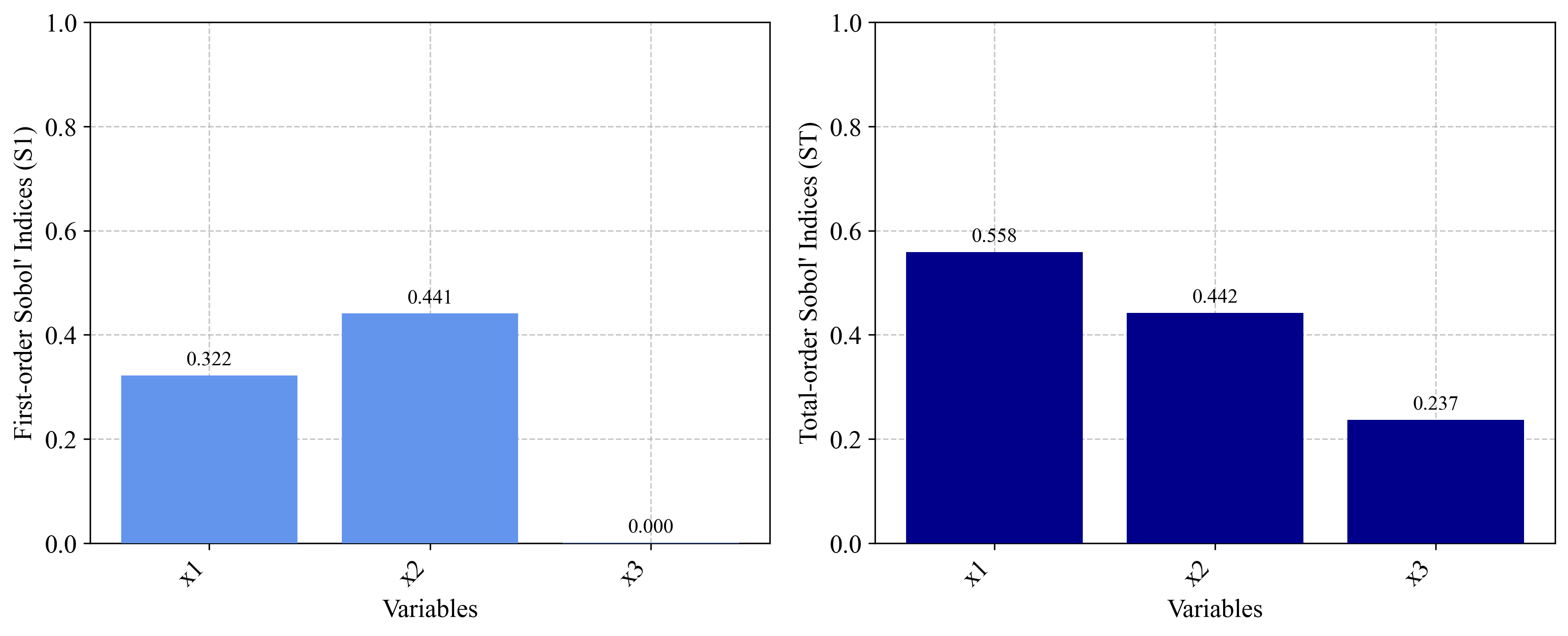
Ishigami Function¶

The Ishigami function is a common benchmark for sensitivity analysis:

import numpy as np
from PyEGRO.sensitivity.SApce import run_sensitivity_analysis

# Define the Ishigami function
def ishigami_function(X):
    """
    Ishigami function - common benchmark for sensitivity analysis.
    """
    a = 7
    b = 0.1

    x1 = X[:, 0]
    x2 = X[:, 1]
    x3 = X[:, 2]

    return np.sin(x1) + a * np.sin(x2)**2 + b * x3**4 * np.sin(x1)

# Define data_info
ishigami_data = {
    'variables': [
        {
            'name': 'x1',
            'vars_type': 'design_vars',
            'distribution': 'uniform',
            'range_bounds': [-np.pi, np.pi],
            'description': 'First variable'
        },
        {
            'name': 'x2',
            'vars_type': 'design_vars',
            'distribution': 'uniform',
            'range_bounds': [-np.pi, np.pi],
            'description': 'Second variable'
        },
        {
            'name': 'x3',
            'vars_type': 'design_vars',
            'distribution': 'uniform',
            'range_bounds': [-np.pi, np.pi],
            'description': 'Third variable'
        }
    ]
}

# Save data_info
import json
import os
os.makedirs("DATA_PREPARATION", exist_ok=True)
with open("DATA_PREPARATION/ishigami_data.json", 'w') as f:
    json.dump(ishigami_data, f)

# Run analysis
results_df = run_sensitivity_analysis(
    data_info_path="DATA_PREPARATION/ishigami_data.json",
    true_func=ishigami_function,
    polynomial_order=6,  # Higher order needed for trigonometric functions
    num_samples=1000,
    output_dir="RESULT_SA_ISHIGAMI",
    show_progress=True
)

# Print results
print("\nIshigami Function Sensitivity Analysis Results:")
print("-" * 50)
print(results_df)

# Validate against known analytical values
print("\nAnalytical Comparison:")
print("First-order indices should be approximately:")
print("x1: 0.314, x2: 0.442, x3: 0.0")
print("Total-order indices should be approximately:")
print("x1: 0.558, x2: 0.442, x3: 0.244")

alt text

↪ Compare with COMSOL results

Rosenbrock Function¶

The Rosenbrock function demonstrates sensitivity analysis on an optimization benchmark:

import numpy as np
from PyEGRO.sensitivity.SApce import run_sensitivity_analysis

# Define the Rosenbrock function
def rosenbrock_function(X):
    """
    Rosenbrock function - common optimization benchmark.

    f(x,y) = (a-x)² + b(y-x²)²
    """
    n_dim = X.shape[1]
    result = 0

    for i in range(n_dim - 1):
        a = 1
        b = 100
        result += (a - X[:, i])**2 + b * (X[:, i+1] - X[:, i]**2)**2

    return result

# Define data_info for 4D Rosenbrock
rosenbrock_data = {
    'variables': [
        {
            'name': 'x1',
            'vars_type': 'design_vars',
            'distribution': 'uniform',
            'range_bounds': [-2, 2],
            'description': 'First dimension'
        },
        {
            'name': 'x2',
            'vars_type': 'design_vars',
            'distribution': 'uniform',
            'range_bounds': [-2, 2],
            'description': 'Second dimension'
        },
        {
            'name': 'x3',
            'vars_type': 'design_vars',
            'distribution': 'uniform',
            'range_bounds': [-2, 2],
            'description': 'Third dimension'
        },
        {
            'name': 'x4',
            'vars_type': 'design_vars',
            'distribution': 'uniform',
            'range_bounds': [-2, 2],
            'description': 'Fourth dimension'
        }
    ]
}

# Save data_info
import json
with open("DATA_PREPARATION/rosenbrock_data.json", 'w') as f:
    json.dump(rosenbrock_data, f)

# Run analysis
results_df = run_sensitivity_analysis(
    data_info_path="DATA_PREPARATION/rosenbrock_data.json",
    true_func=rosenbrock_function,
    polynomial_order=5,
    num_samples=1000,
    output_dir="RESULT_SA_ROSENBROCK",
    show_progress=True
)

# Print results
print("\nRosenbrock Function Sensitivity Analysis Results:")
print("-" * 50)
print(results_df)

# Calculate interaction effects
interaction_effect = results_df['Total-order'] - results_df['First-order']
results_df['Interaction_Effect'] = interaction_effect

# Print interaction analysis
print("\nVariable Interaction Analysis:")
for i, row in results_df.iterrows():
    if row['Interaction_Effect'] > 0.1:
        print(f"{row['Parameter']}: Strong interaction effect ({row['Interaction_Effect']:.4f})")
    elif row['Interaction_Effect'] > 0.01:
        print(f"{row['Parameter']}: Moderate interaction effect ({row['Interaction_Effect']:.4f})")
    else:
        print(f"{row['Parameter']}: Weak interaction effect ({row['Interaction_Effect']:.4f})")

Borehole Function¶

The borehole function is a common benchmark in engineering sensitivity analysis:

import numpy as np
from PyEGRO.sensitivity.SApce import run_sensitivity_analysis

# Define the borehole function
def borehole_function(X):
    """
    Borehole function - models water flow through a borehole.
    """
    rw = X[:, 0]  # radius of borehole (m)
    r = X[:, 1]   # radius of influence (m)
    Tu = X[:, 2]  # transmissivity of upper aquifer (m²/year)
    Hu = X[:, 3]  # potentiometric head of upper aquifer (m)
    Tl = X[:, 4]  # transmissivity of lower aquifer (m²/year)
    Hl = X[:, 5]  # potentiometric head of lower aquifer (m)
    L = X[:, 6]   # length of borehole (m)
    Kw = X[:, 7]  # hydraulic conductivity of borehole (m/year)

    numerator = 2 * np.pi * Tu * (Hu - Hl)

    denominator = np.log(r / rw) * (1 + (2 * L * Tu) / (np.log(r / rw) * rw**2 * Kw) + Tu/Tl)

    return numerator / denominator

# Define data_info
borehole_data = {
    'variables': [
        {
            'name': 'rw',
            'vars_type': 'design_vars',
            'distribution': 'uniform',
            'range_bounds': [0.05, 0.15],
            'description': 'Radius of borehole (m)'
        },
        {
            'name': 'r',
            'vars_type': 'design_vars',
            'distribution': 'uniform',
            'range_bounds': [100, 50000],
            'description': 'Radius of influence (m)'
        },
        {
            'name': 'Tu',
            'vars_type': 'env_vars',
            'distribution': 'uniform',
            'low': 63070, 
            'high': 115600,
            'description': 'Transmissivity of upper aquifer (m²/year)'
        },
        {
            'name': 'Hu',
            'vars_type': 'env_vars',
            'distribution': 'uniform',
            'low': 990, 
            'high': 1110,
            'description': 'Potentiometric head of upper aquifer (m)'
        },
        {
            'name': 'Tl',
            'vars_type': 'env_vars',
            'distribution': 'uniform',
            'low': 63.1, 
            'high': 116,
            'description': 'Transmissivity of lower aquifer (m²/year)'
        },
        {
            'name': 'Hl',
            'vars_type': 'env_vars',
            'distribution': 'uniform',
            'low': 700, 
            'high': 820,
            'description': 'Potentiometric head of lower aquifer (m)'
        },
        {
            'name': 'L',
            'vars_type': 'design_vars',
            'distribution': 'uniform',
            'range_bounds': [1120, 1680],
            'description': 'Length of borehole (m)'
        },
        {
            'name': 'Kw',
            'vars_type': 'env_vars',
            'distribution': 'uniform',
            'low': 9855, 
            'high': 12045,
            'description': 'Hydraulic conductivity of borehole (m/year)'
        }
    ]
}

# Save data_info
import json
with open("DATA_PREPARATION/borehole_data.json", 'w') as f:
    json.dump(borehole_data, f)

# Run analysis
results_df = run_sensitivity_analysis(
    data_info_path="DATA_PREPARATION/borehole_data.json",
    true_func=borehole_function,
    polynomial_order=3,
    num_samples=1000,
    output_dir="RESULT_SA_BOREHOLE",
    show_progress=True
)

# Print results
print("\nBorehole Function Sensitivity Analysis Results:")
print("-" * 50)
print(results_df.sort_values('Total-order', ascending=False))

# Identify key parameters
top_params = results_df.sort_values('Total-order', ascending=False).head(3)['Parameter'].tolist()

print("\nBorehole Analysis Insights:")
print(f"Most influential parameters: {', '.join(top_params)}")
print("\nEngineering Recommendations:")
for param in top_params:
    print(f"- Focus on accurate measurement and control of {param}")

Circuit Design Problem¶

This example demonstrates sensitivity analysis for an electronic circuit design:

import numpy as np
from PyEGRO.sensitivity.SApce import run_sensitivity_analysis

# Define a circuit model (RC low-pass filter)
def circuit_performance(X):
    """
    Calculate the cutoff frequency and performance metrics of an RC filter.

    Variables:
    - R1: Resistor 1 value (ohms)
    - R2: Resistor 2 value (ohms)
    - C1: Capacitor 1 value (farads)
    - C2: Capacitor 2 value (farads)
    - f: Frequency of interest (Hz)
    """
    R1 = X[:, 0]
    R2 = X[:, 1]
    C1 = X[:, 2]
    C2 = X[:, 3]
    f = X[:, 4]

    # Impedances
    Z_R1 = R1
    Z_R2 = R2
    Z_C1 = 1 / (2j * np.pi * f * C1)
    Z_C2 = 1 / (2j * np.pi * f * C2)

    # Parallel combination of R2 and C2
    Z_parallel = (Z_R2 * Z_C2) / (Z_R2 + Z_C2)

    # Series with R1 and C1
    Z_total = Z_R1 + Z_C1 + Z_parallel

    # Calculate transfer function magnitude
    H = Z_parallel / Z_total
    gain_dB = 20 * np.log10(np.abs(H))

    # For sensitivity analysis, use the absolute gain loss
    return -gain_dB

# Define data_info
circuit_data = {
    'variables': [
        {
            'name': 'R1',
            'vars_type': 'design_vars',
            'distribution': 'normal',
            'range_bounds': [980, 1020],  # 1kΩ with 2% tolerance
            'cov': 0.02,
            'description': 'Resistor 1 (ohms)'
        },
        {
            'name': 'R2',
            'vars_type': 'design_vars',
            'distribution': 'normal',
            'range_bounds': [9800, 10200],  # 10kΩ with 2% tolerance
            'cov': 0.02,
            'description': 'Resistor 2 (ohms)'
        },
        {
            'name': 'C1',
            'vars_type': 'design_vars',
            'distribution': 'normal',
            'range_bounds': [9.5e-9, 10.5e-9],  # 10nF with 5% tolerance
            'cov': 0.05,
            'description': 'Capacitor 1 (farads)'
        },
        {
            'name': 'C2',
            'vars_type': 'design_vars',
            'distribution': 'normal',
            'range_bounds': [9.5e-9, 10.5e-9],  # 10nF with 5% tolerance
            'cov': 0.05,
            'description': 'Capacitor 2 (farads)'
        },
        {
            'name': 'f',
            'vars_type': 'env_vars',
            'distribution': 'uniform',
            'low': 1000,
            'high': 10000,
            'description': 'Frequency (Hz)'
        }
    ]
}

# Save data_info
import json
with open("DATA_PREPARATION/circuit_data.json", 'w') as f:
    json.dump(circuit_data, f)

# Run analysis
results_df = run_sensitivity_analysis(
    data_info_path="DATA_PREPARATION/circuit_data.json",
    true_func=circuit_performance,
    polynomial_order=4,
    num_samples=800,
    output_dir="RESULT_SA_CIRCUIT",
    show_progress=True
)

# Print results
print("\nCircuit Design Sensitivity Analysis Results:")
print("-" * 50)
print(results_df.sort_values('Total-order', ascending=False))

# Electronics design insights
top_params = results_df.sort_values('Total-order', ascending=False).head(2)['Parameter'].tolist()

print("\nCircuit Design Insights:")
print(f"Most influential parameters: {', '.join(top_params)}")
print("\nDesign Recommendations:")
for param in top_params:
    if param in ['R1', 'R2']:
        print(f"- Use precision resistors for {param} with tighter tolerance")
    elif param in ['C1', 'C2']:
        print(f"- Use high-stability capacitors for {param} (e.g., film instead of ceramic)")
    elif param == 'f':
        print("- Design the circuit for the specific frequency range of interest")